Correlation
Difference between cor() and cor.test()
The cor() function will calculate:
- a correlation between 2 variables
- a correlation matrix between more than 2 variables
Among statisticians there are 3 popular opinions about the choice of correlation coefficient.
1. it depends on the type of data:
- continuous measurements -> Pearson correlation
- discrete measurements or ranked categories -> Kendall or Spearman correlation
2. it depends on normality:
- normally distributed, continuous measurements -> Pearson correlation
- continuous measurements that are not normally distributed, discrete measurements or ranked categories -> Kendall or Spearman correlation
3. it depends on the relation between the 2 variables:
- linear -> Pearson correlation
- monotonic -> Kendall or Spearman correlation
See this blog for an explanation on the difference between a linear and a monotonic relation.
The cor.test() function will only work on 2 variables, not on more than 2 variables. It will calculate:
- correlation coefficient
- p-value that defines if this correlation is significantly different from 0
Normality is important here, especially multivariate normality:
- multivariate normality -> Pearson
- no multivariate normality -> Kendall or Spearman
Warning when you use Kendall or Spearman
You will see this warning every time you do a non-parametric test. It tells you that these tests do not work well when there are ties in your data (= the same value appearing multiple times in the data set).
cor.test(mtcars$mpg,mtcars$wt,method="kendall")

data: mtcars$mpg and mtcars$wt
z = -5.7981, p-value = 6.706e-09
alternative hypothesis: true tau is not equal to 0
sample estimates:
tau
-0.7278321

Warning message:
In cor.test.default(mtcars$mpg, mtcars$wt, method = "kendall") :
Cannot compute exact p-value with ties
Output in APA style
You can write the correlation matrix to a document in APA style:
library(apaTables)
apa.cor.table(mtcars[1:5],filename="Table1_APA.doc",table.number=1)
will generate a word document in your working directory with the following content:
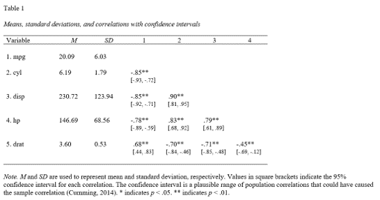
Add correlation coefficient to the scatter plot
To add the correlation coefficient to a plot use the ggpubr package. First create the scatter plot.
library(ggplot2)
p <- ggplot(mtcars,aes(hp,mpg)) + geom_point()
Then add a regression line and the Pearson correlation coefficient.
library(ggpubr)
p + geom_smooth(method="lm",se=FALSE) + stat_cor(method="pearson")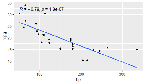
Pearson correlation coefficient and p-value of cor.test() are automatically added to the plot.
Linear transformations will not change the correlation coefficient
Linear transformation (+k, -k, *k, /k where k is a constant) will not change the correlation.
p2 <- ggplot(mtcars,aes(hp+100,mpg)) + geom_point()
p2 + geom_smooth(method="lm",se=FALSE) + stat_cor(method="pearson")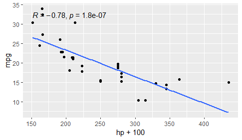
p3 <- ggplot(mtcars,aes(hp,mpg*2)) + geom_point()
p3 + geom_smooth(method="lm",se=FALSE) + stat_cor(method="pearson")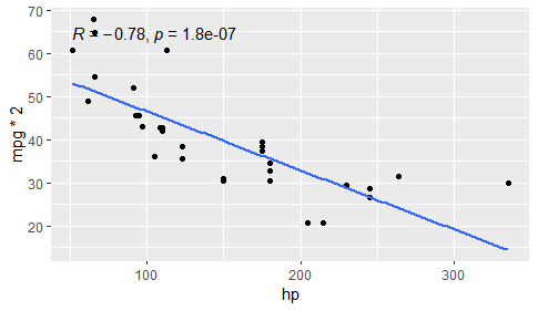
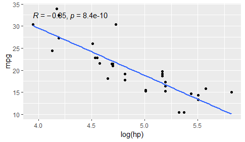
Non-linear transformations can improve the correlation coefficient
A non-linear transformation (log, square root…) can improve the correlation provided the relation between X and Y is non-linear. Check the scatter plot to see if there is a non-linear relation between X and Y. If the relation looks linear don’t do a non-linear transformation.
p4 <- ggplot(mtcars,aes(log(hp),mpg)) + geom_point()
p4 + geom_smooth(method="lm",se=FALSE) + stat_cor(method="pearson")